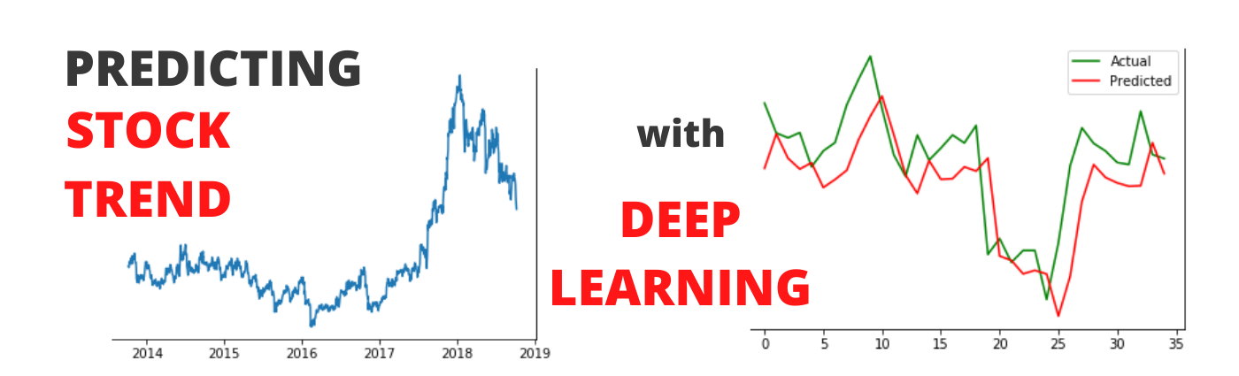
Predicting Stock Trend Using Deep Learning

Predicting the upcoming trend of stock using Deep learning Model(Recurrent Neural Network)

In this article, we will build a deep learning model (specifically the RNN Model) that will help us to predict whether the given stock will go up or down in the future. Remember, we are not interested in predicting the actual values as that will be far more complex compared to the prediction of the trend.

If you are new to deep learning, don’t worry I will try my best to give a simple and easy explanation of the whole tutorial. Also, I consider this particular project as an entry-level project or the simplest project that one must do with the recurrent neural networks.

So, the first question that comes in mind is What is Recurrent Neural Network?

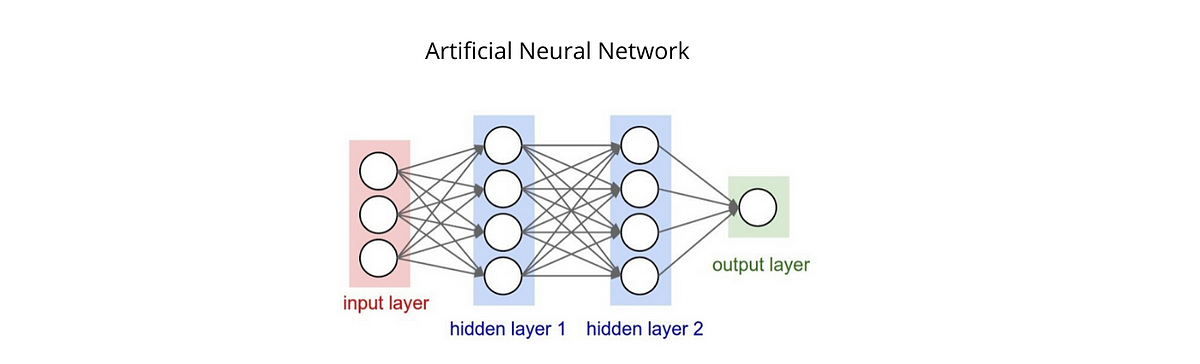
To understand this, we have to understand the neural network first. Here, I assume that you are already familiar with machine learning. The neural network, also known as Artificial Neural Network (ANN), is made up of three stages namely the input layer, the number of hidden layers, and the output layer. As the name suggests, the input layer is used to take input and feed it into the model, and the output layer is used to gives the predicted outcome whereas the hidden layers are responsible for all mathematical computations(every unit or cell is responsible for doing small operations ). Know more about ANN here.

Recurrent Neural Networks(RNN) are one of the types of neural networks in which the output of one step in time act as the input for the next step in time. For example, in the sentence “I am hungry, I need food”, it is very important to remember the word hungry to predict food. Hence to predict the upcoming word, it is important to remember the previous words. And to resolve this kind of problem, RNN comes to rescue. The main feature of RNN is a hidden state that remembers the sequence information. RNN performs very well when it comes to sequence data like weather, stock market, text, etc. I will not go in great detail about the working of the RNN considering that the article is beginners friendly, but you can always Google things 😄

Prerequisites:-

I assume that you are familiar with python and already have installed the python 3 in your systems. I have used a jupyter notebook for this tutorial. You can use the IDE of your like.

Dataset Used:-

The dataset that we have used for this tutorial is of NSE Tata Global stock and is available on GitHub.

Installing Required Libraries

For this project, you need to have the following packages installed in your python. If they are not installed, you can simply usepip install PackageName .

• NumPy — This library provides fast computing n-dimensional array objects.
• pandas — It provides a data frame and series to perform manipulation and analysis on data.
• matplotlib — This library helps in the visualization of data using various plots.
• scikit-learn — It is a machine learning library that provides various tools and algorithms for predictive analysis. We will use its tools or functions for the preprocessing of the data.
• Keras — It is a high level deep learning library built over TensorFlow to provide a simple implementation of neural networks. We have used it because it is beginners friendly and easy to implement.
• TensorFlow — This library is required by the Keras as Keras runs over the TensorFlow itself.

LETS START CODING

Firstly, we need to import the libraries that we will use in the project. Here, numpy is used to create NumPy arrays for training and testing data. pandas for making the data frame of the dataset and retrieving values easily. matplotlib.pyplot to plot the data like overall stock prices and predicted prices. MinMaxScaler from sklearn’s(scikit-learn) preprocessing package to normalize the data. We have imported Sequential dense LSTM Dropoutfrom Keras that will help to create a deep learning model. We will discuss these modules later on.

import numpy as np
import pandas as pd
import matplotlib.pyplot as plt
from sklearn.preprocessing import MinMaxScaler
#for deep learning model
from keras import Sequential
from keras.layers import Dense
from keras.layers import LSTM
from keras.layers import Dropout

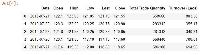
Now, we have loaded our dataset as a data frame in a variable named df. Then, we have checked the shape of the dataset that comes out to be (2035,8) means there are 2035 rows and 8 columns in the dataset. After that, we have reversed the dataset upside-down so that the date starts from the oldest and goes to the most recent, and in doing so we also have to reset our indexes as well. Then we have just printed some starting rows of the dataset with head() . The first 5 entries of dataset are shown in screenshot below.

df = pd.read_csv('NSE-TATAGLOBAL.csv')
df.shape
df = df[::-1]
df = df.reset_index(drop=True)
df.head()

​

We have chosen only one feature that is Open to train our model but you are free to choose more than one feature but then the code will be changed accordingly. In the training set, we have 2000 values while in testing we decided to have only 35. Then we simply printed the shape of both train_set test_set that comes out to be (2000,1) and (35,1) respectively.

open_price = df.iloc[:,1:2]
train_set = open_price[:2000].values
test_set = open_price[2000:].values
print("Train size: ",train_set.shape)
print("Test size:",test_set.shape)

Here, we have converted the Date column into DateTime format to plot it conveniently. Then simply used plot_date to plot the figure of the open price of stock throughout the time line and saved the figure using savefig .

dates = pd.to_datetime(df['Date'])
plt.plot_date(dates, open_price,fmt='-')
plt.savefig("test1final.png")

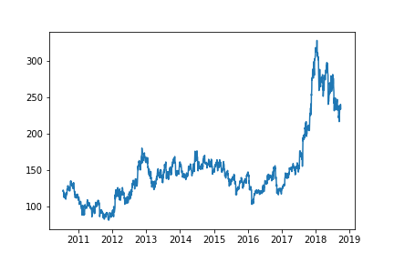
​ Open price of NSE Tata Global (2010–2019)

Now, we have initialized the MinMaxScalar that is used to scale every value in the range of 0 and 1. It is a very important step because Neural Networks and other algorithms converge faster when features are on a relatively similar scale.

sc = MinMaxScaler()
train_set_scaled = sc.fit_transform(train_set)

Here comes the tricky part. Now, we have to make the data suitable for our RNN model i.e. making sequences of data with the target final value. Let me explain with the example. Suppose we have a dataset that has values from 1–10, and we have a sequence length of 3. In that case, our training data will look like this-

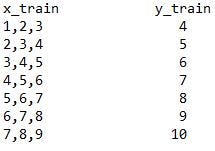
​ Example of sequence training data

Here in the code, the length of the sequence is 60 that means only the previous 60 values will decide the next value, not the whole dataset. After that, we have created NumPy arrays of both x_train and y_train for fast computation and reshaped the training set according to the requirement of our model. The final shape of x_train comes out to be (1940, 60, 1).

x_train = []
y_train = []
for i in range(60,2000):
    x_train.append(train_set_scaled[i-60:i,0])
    y_train.append(train_set_scaled[i,0])
x_train = np.array(x_train)
y_train = np.array(y_train)
x_train = np.reshape(x_train,(x_train.shape[0],x_train.shape[1],1))
x_train.shape

Now, we will create our model’s architecture. We have used Keras because it is quite easy to make a deep learning model with Keras compared to other available libraries. Here, we have initialized our Sequential object that acts as the bundler for all the layers inside the model. Our model in total has 4 LSTM layers and one dense layer.

LSTM(Long Short Term Memory) is a type of recurrent neural network that has some contextual state cells that act as long-term or short-term memory cells and these cells modulate the output. It is important when we need to predict the output based on the historical context rather than just the last input. For example, we have to predict the next number in the sequence 3,4,5,? then output is simply 6(x+1) but in the sequence 0,2,4,? the output is also 6 but it also depends on contextual information.

Dropout is used to prevent the over fitting of the data by simply deactivating some of the units(neurons) at a time, In our case, 20% of units are deactivated at a time. In the end, we have a Dense layer with 1 unit that gives the predicted value. Then, we simply compiled our model with adam optimizer and fit our model on the data and run for 20 iterations i.e. epochs .

reg = Sequential()
reg.add(LSTM(units = 50,return_sequences=True,input_shape=(x_train.shape[1],1)))
reg.add(Dropout(0.2))
reg.add(LSTM(units = 50,return_sequences=True))
reg.add(Dropout(0.2))
reg.add(LSTM(units = 50,return_sequences=True))
reg.add(Dropout(0.2))
reg.add(LSTM(units=50))
reg.add(Dropout(0.2))
reg.add(Dense(units=1))
reg.compile(optimizer = 'adam',loss='mean_squared_error')
reg.fit(x_train,y_train, epochs=20, batch_size =1,verbose=2)

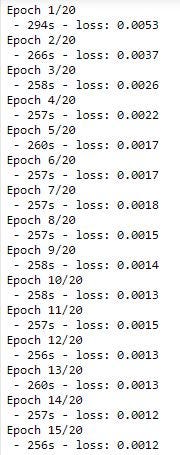
​ Loss of every iteration

As you can see our model converges at 15 epochs and it took me around 90 minutes to run 20 epochs in total. Yes RNN model takes time to train.

​ RNN Model Takes Time

Now, its time to create input for the testing. The shape of input is (95, 1) and we scale this data as well.

input = open_price[len(open_price)-len(test_set)-60:].values
input.shape
input = sc.transform(input)

Here’s the final part, in which we simply make sequences of data to predict the stock value of the last 35 days. The first sequence contains data from 1–60 to predict 61st value, second sequence 2–61 to predict 62nd value, and so on. The shape of x_test is (35, 60, 1) that justifies the explanation.

x_test = []
for i in range(60,95):
    x_test.append(input[i-60:i,0])
x_test = np.array(x_test)
x_test = np.reshape(x_test,(x_test.shape[0],x_test.shape[1],1))
x_test.shape

In the end, we simply predict the values using predict the function of our defined model and plot the last 35 actual and predicted values of a given stock.

pred = reg.predict(x_test)
pred = sc.inverse_transform(pred)
plt.plot(test_set,color='green')
plt.plot(pred,color='red')
plt.title('Stock_prediction')
plt.show()

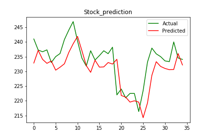
​ Final Result

As you can see from the figure itself, our model was quite accurate in predicting the upcoming trend of the given stock.😎 Now you can become a great advisor in the share market. 😆

The source code is available on GitHub. Please feel free to make improvements.

The model can further be improved by incorporating more features, increasing the dataset, and tuning the model itself.

Thank you for your precious time.😊And I hope you like this tutorial.